Science case difference between 2Hz cut-off and 10Hz cut-off
main selling points for as low frequencies as possible:
- early warning with sky localization for EM followup thanks to early SNR buildup. ~1000s-10ks
- IMBHs/IMRIs with higher total masses (>1000Msun) and up to high redshifts → cosmic history of SMBH seeds
- Long inspiral gives highly improved CBC parameter estimation even with just small SNR gains, breaking degeneracies with precession and higher modes, constraining ellipticity before it is completely radiated away. → formation channels and environments
- No other observatory will look at this range, except maybe DECIGO on even longer timescales → unique discovery potential for unknown unknowns.
For many more analyses low frequencies yield improved rates/sensitivity/precision, but it can usually be offset with increased bucket sensitivity instead; the three above seem to be the main drivers for low-freq specifically.
CBC
early warning and sky localization
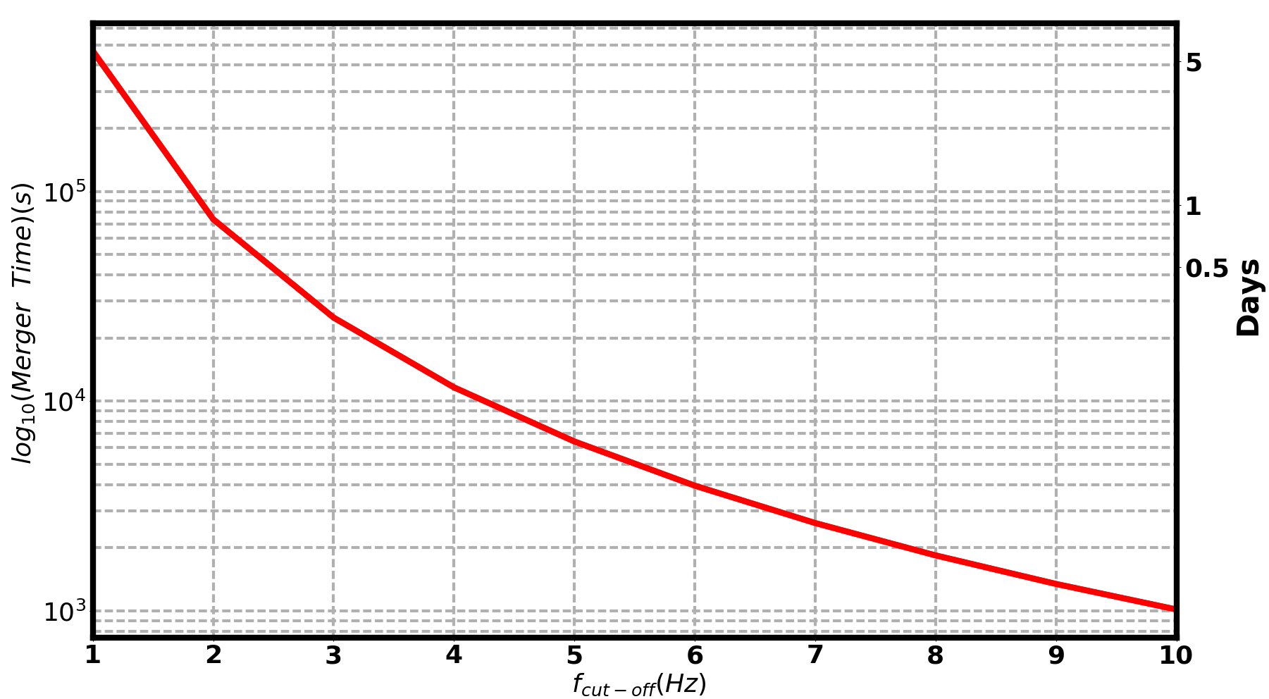
- Lifetime in the detector window: ignoring SNR buildup for the moment, total BNS track length increases from ~10 minutes for 10Hz lower cutoff to ~1 day at 2Hz cutoff. [Plot: M. Chan]
- For a useful early warning alert, we also want good sky localisation early enough. See below.
- More specifically, we want the time before coalescence that some SNR (or false-alarm rate) threshold is crossed. Using universal SNR distribution and an estimated merger rate (or fancier: redshift-dependent distribution+rate), can predict number of events as a function of pre-alert time.
- This FoM, from Adhikari et al, LIGO-P1700208 for LIGO Voyager, red is the only Voyager variant with some sensitivity below 10Hz. Note the localization panel assumes 2x Voyager + 1x aVirgo.

- Localisation accuracy also improves when starting at lower frequency, and can actually be done surprisingly well with a single-site ET for sources that are close enough. (The daily rotation of the detector gives “synthetic aperture”, i.e. equivalent to a network.
- Below is a plot showing the localisation by an L-shape ET or CE for the same source at a location randomly selected but at three different distances.
- The signal starts at 1Hz, and the two detectors (ET and CE) are assumed to be at the same location for a fair comparison.
- The top panel of the plot is for ET and the bottom panel is for CE.
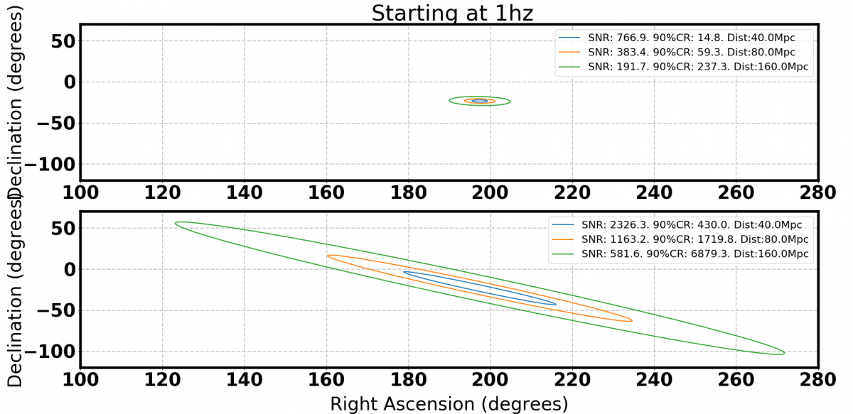
- It can be seen that although CE accumulates much higher SNR, the localistion by L-shape ET is much smaller because ET's improvement in the low frequency band provides a long in-band duration of the signal.
- Thus, if with the early alerts to EM followers, we need low-frequency sensitivity.
- In addition, given the localization, polarization measurement from ET topology gives you source inclination too.

going to high BH masses and redshifts
- The lower the frequency, the higher the BH masses we probe. fLSO ~ 4400 / ( Mtot[Msun] * (1+z) )
- We measure redshifted detector frame masses. → meaning higher cosmological reach
- Intermediate mass black holes (IMBHs) could be observed both as IMBH-IMBH binaries and as IMRIs with stellar-mass BHs or NSs.
- Observing IMBH/BBH at higher redshifts probes the BBH formation history and mass function evolution –> cosmology, galaxy formation!
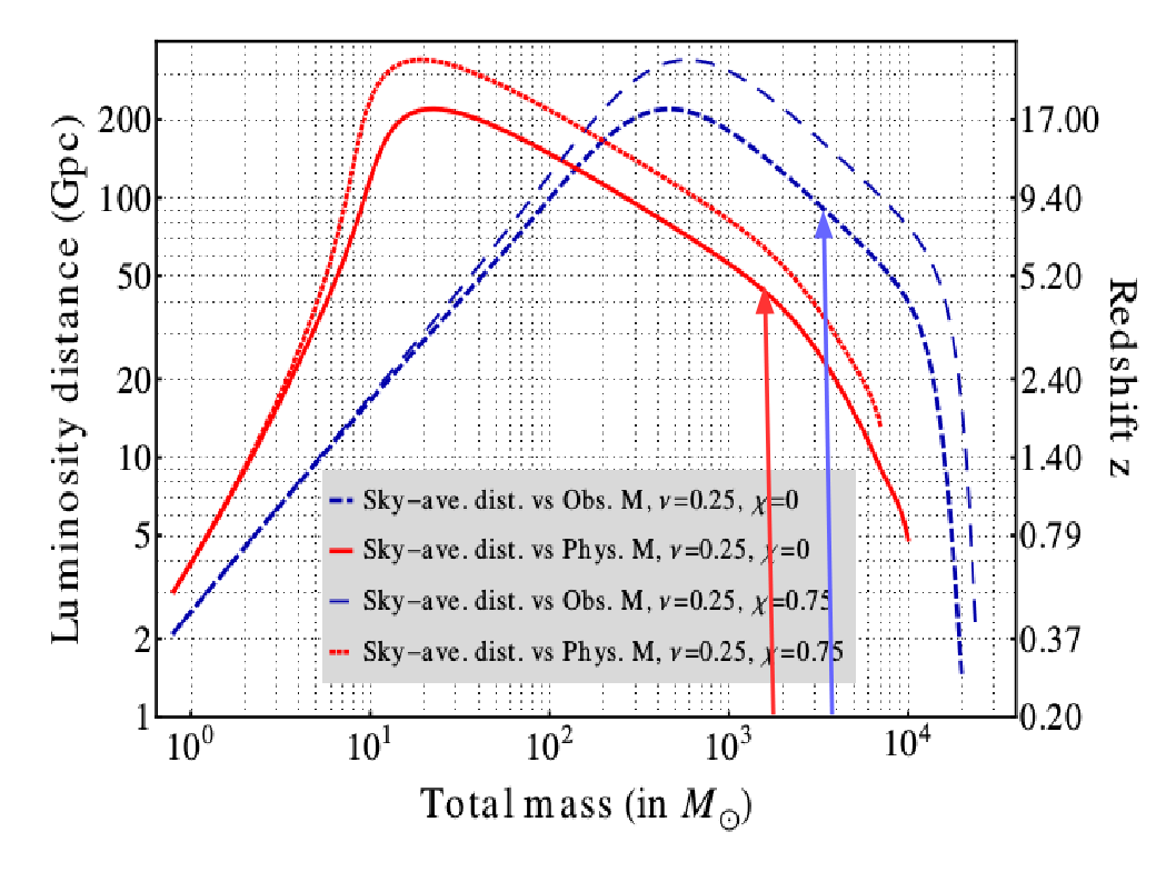 the arows indicate the highest masses we woud detect if we reduced the sensitivity to 10Hz. [Sathya et al 2012]
- IMRIs have rich waveforms, allowing e.g. additional TGR opportunities.
Parameter Estimation from long inspirals
- Already for a basic quantity like chirp mass, low freqs may contribute only few % of SNR, but large improvements in PE. From Salvo's talk this week, how well CE can do, need to quantify low-freq ET in comparison:

- Higher order effects in BBH that might be much better observable with very long inspirals:
- precession
- eccentricity (gets radiated away until late inspiral, really need as early as possible)
- higher multipole modes (more prominent for higher mass ratio, profits from being able to see higher-Mtot systems)
- Observing BBH at higher redshifts. BBH formation history, mass function evolution - need to quantify.
Testing GR
- long inspiral will let us see some deviations from GR with higher sensitivity: (references?)
- speed of gravity / LIV tests particularly helped by high-redshift sources, too
- parametrized PN-violation tests should be helped by many cycles
- though for many tests: do low-freq cycles help by themselves, or can be easily made up for by high SNR from bucket?
- BNS: tidal deformability? Both intuition and Table 1 of Adhikari et al imply bucket/high-freq more relevant, but comparing the non-deformed early inspiral with the deformed late inspiral might be quite useful, at the very least to study degeneracies/systematics. Need an actual expert to look into whether this is relevant early enough in the inspiral for low freqs to matter at all.
- remember tradeoffs with high-freq, interesting things like post-merger and BNS studies require high-freq as well!
Stochastic Backgrounds
- cosmic background from BH/ and NS binaries: low frequencies are very important
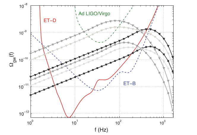 Lots of sensitivity for the GW background at low frequencies. The expected spectrum is a power law but the level
is determined by the integrated rate density. Probably by 2030 we will have a very good idea of
the level of the background from binaries.
Lots of sensitivity for the GW background at low frequencies. The expected spectrum is a power law but the level
is determined by the integrated rate density. Probably by 2030 we will have a very good idea of
the level of the background from binaries.
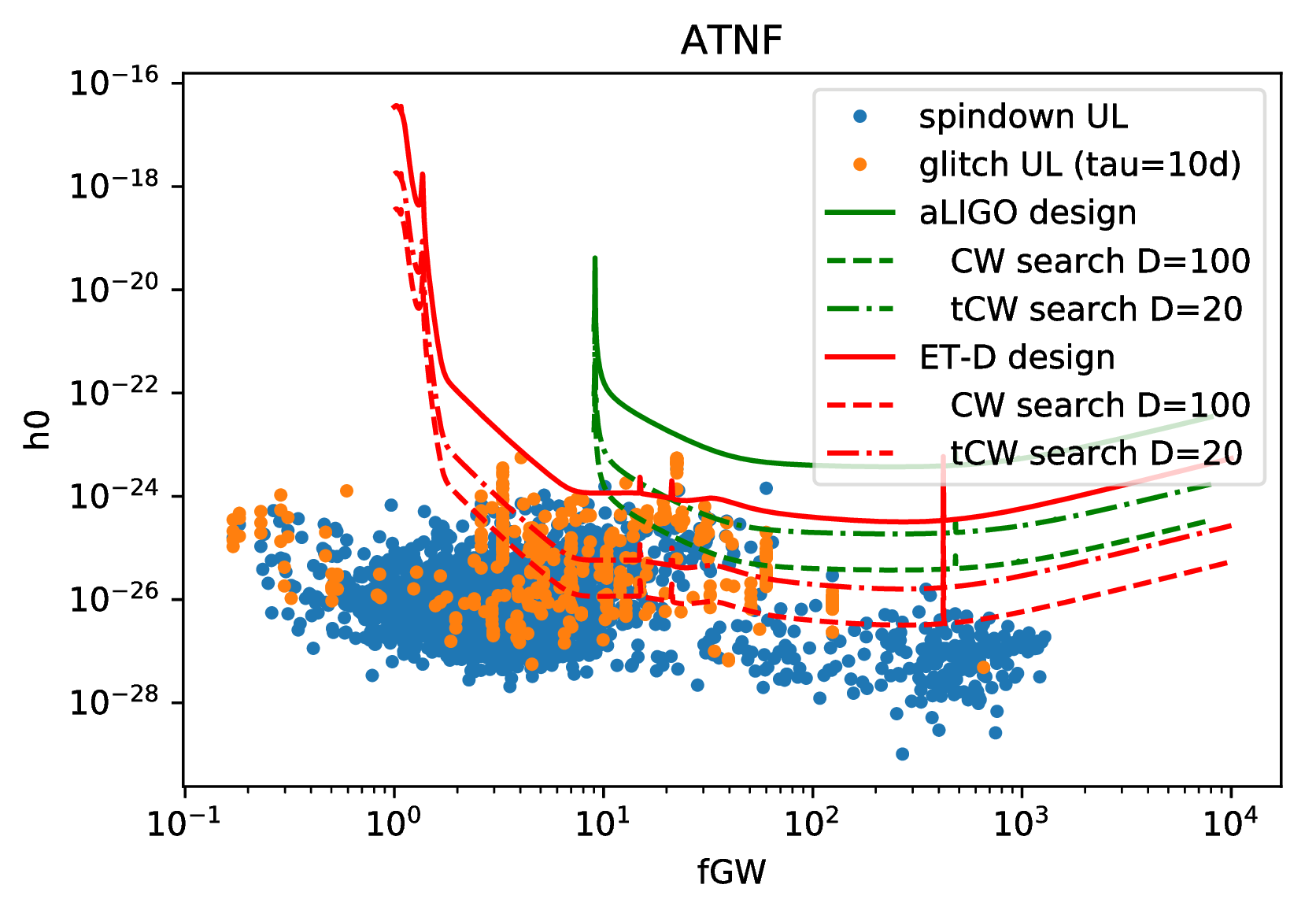
Continuous Waves from Neutron Stars
- Most of the bulk of known pulsars population is at low frequencies.
- Including particularly glitchy ones that could make good transient emitters!
- Preliminary estimate: could beat spindown upper limit for ~350 known pulsars from ATNF with full ET-D curve, ~150 left with hard cut at 10 Hz. (Pitkin 2011 estimated ~100–600 observable with ET-C)
- We don't know of any lower limit of NS ellipticities or how GW emission really correlates with source properties, so we should just aim to have as many interesting objects in band as possible/
- Blind searches are also potentially sensitive to EM-dark NSs, but unclear whether “horizontal” or “vertical” extension of search space is more promising.
- CW ULs from known pulsars and glitches - quick work [D. Keitel], might be a few factors off, but right ballpark:
Supernovae
- rare sources anyway
- core collapse basically emit inside the LIGO band, not much from low freq
- SNIa might have some emission at <1Hz, but very low local rate
- for this source we actually want as much high-freq sensitivity as possible!
resources
- LIGO Voyager blue/red/green: https://dcc.ligo.org/P1700208-v1

- Sathya et al 2012 ET science objectives: https://inspirehep.net/record/1116935
to-do list
All of the following is basically quantitative comparisons that will be equally useful for any other 2G+/3G proposals, so it will be useful to distribute labor in the international 3G science case working group.
- reproduce and extend Table 1 from P1700208:
- IMBH maximum mass, range/horizon
- sky localization (average/cumdist/…, time for early localization)
- spins, precession, eccentricity parameter estimation
- …
- stoch. background: update/verify plot above with current rate knowledge
- full quantitative analysis of early warning / sky localization (Mervin; also do our version of Fig. 6 from P1700208)
- study and quantify influence of many low-freq cycles on tidal estimates (vs. just more SNR overall)
- our version of Salvo's Mchirp plot with low-freq
- update / double-check CW estimates, compare with Matt's 2011 paper
- testing GR: first step is to talk to experts